Linux tutorial
Download the workflow: SPARTA for Linux
- Introduction
- Basic Terminal Commands
- Install Dependencies
- Initializing SPARTA
- Analyzing Example Data
- Analyzing Your Data
- Identifying Potential Batch Effects
- Altering Workflow Execution Options
Introduction
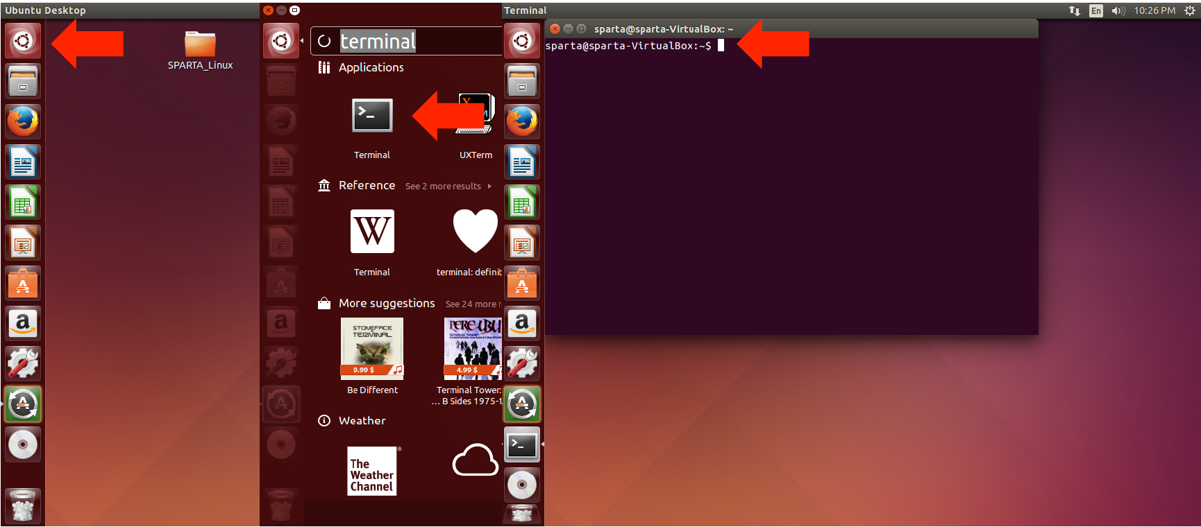
Many bioinformatics software packages and workflows require the user to utilize them from the command line or terminal. SPARTA is no different. The reason the command line interface is utilized is that a great deal of power and flexibility can be gained without the use of a graphical user interface (GUI). Further, a GUI can be difficult to implement across various platforms. To find the command line interface/Terminal on Linux (shown in Ubuntu with red arrows), go to “Search your computer and online sources” button -> Search for “terminal” -> Click on Terminal -> Terminal is now open and ready to enter commands (might just be worth dragging it onto your dock).
Decompress the SPARTA_Linux-master.zip file by clicking on it and extracting all the files to the desktop.
SPARTA expects either compressed (.gz) or uncompressed FASTQ files (.fq or .fastq) as input, with a reference genome file in FASTA format and a genome feature file (.gtf) within the folder that contains the input data. To see an example of appropriate input data, look inside the ExampleData folder within the SPARTA_Linux-master folder.
To download a reference genome and genome feature file for your favorite bacteria, go to the Ensembl website. The reference genome and feature file are already present for the ExampleData.
Basic Terminal Commands
Let’s have a look at some basic Terminal commands, we will cover the commands necessary to:
1. Move through folders
2. List the contents of a folder
3. Make new folders
4. Rename files/folders
5. Delete files/folders
| Command | What it does | Examples | |
|---|---|---|---|
| 1. | cd | Change directory/folder | cd ~ (this changes to your home directory); cd .. (this goes back one folder) |
| 2. | ls | List the contents of a folder | ls |
| 3. | mkdir | Make a new directory/folder | mkdir NewFolder (this will make a new folder called ‘NewFolder’ in your current directory) |
| 4. | mv | Rename or move a file from one name to another | mv file1 file2 (this will rename/move file1 to file2) |
| 5. | rm | Remove a file (add the -r flag to remove a folder) | rm file1 (remove file1); rm -r folder1 (remove folder1) |
Command reference sheet
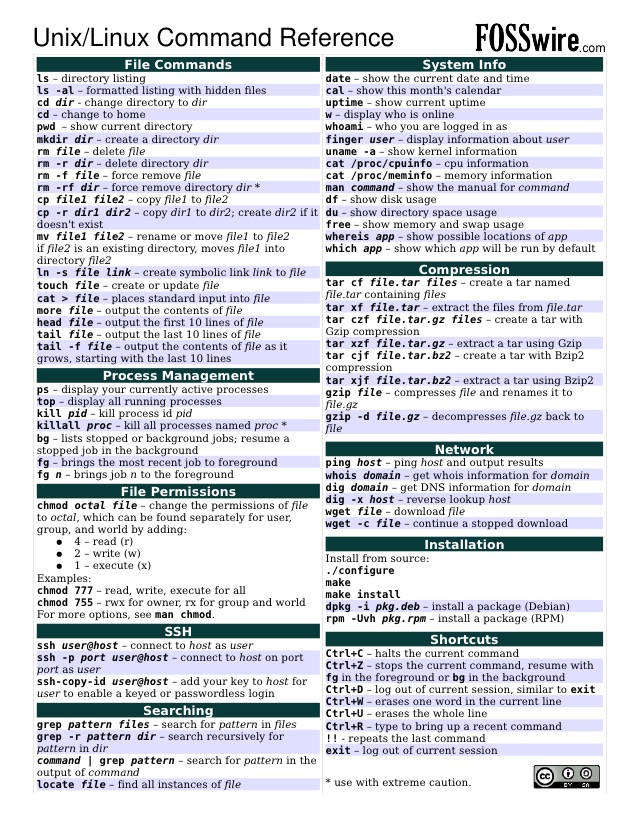
Ref. sheet from: http://files.fosswire.com/2007/08/fwunixref.pdf
Install Dependencies
The SPARTA workflow requires a few things in order to run: Python, Java, NumPy, and R. If you already have these installed, great! If you don’t, let’s start by downloading and installing the dependencies by running the bash script called “install_dependencies.sh”.
To run this script, navigate to the SPARTA_Linux-master folder on the desktop:
cd ~/Desktop/SPARTA_Linux-master
Now, type:
bash install_dependencies.sh
This will update, download, and install the necessary dependencies to run SPARTA.
Congratulations! You’ve installed the necessary dependencies to run SPARTA!
Initializing SPARTA
Once SPARTA is initialized, the workflow will seek to identify that all of the necessary dependencies are met. If they are not satisfied, a message specific to what is not installed will appear as output in the terminal window.
To initialize SPARTA, go to the Terminal and navigate to the SPARTA_Linux-master folder on your desktop by typing:
cd ~/Desktop/SPARTA_Linux-master
To start the workflow, type:
python SPARTA.py
This will start the software and check for dependencies.
Analyzing Example Data
SPARTA is distributed with some example data. Specifically, it is the first 100,000 reads of each sample from Baker et al..
To begin the analysis, navigate into the SPARTA_Linux-master folder and drag and drop the folder called “ExampleData” out onto the desktop.
If you haven’t already, initialize SPARTA from the Terminal.
If all the dependencies are met, SPARTA will pause and prompt the user:
Is the RNAseq data in a folder on the Desktop? (Y or N):
Type:
Y
Hit Enter/Return
Note
SPARTA assumes the data is located in a folder on the desktop by default. It is easiest if all future analyses have the data in a folder (WITHOUT SPACES IN THE NAME) on the desktop.
Now it will prompt the user for the name of the folder:
What is the name of the folder on the Desktop containing the RNAseq data?:
Type:
ExampleData
This is the name of the folder on the desktop that contains the input example data. Hit Enter/Return. From here, the software will trim, QC, align, and count transcript abundance for each sample. All output/analyses are put in a folder that SPARTA generates on the desktop called “RNAseq_Data”. Within this folder are separate folders for each SPARTA run that are denoted by the date (e.g. 2015-06-04). Within these folders are four more folders that separate each step of the analysis and are called: 1) QC, 2) Bowtie, 3) HTSeq, and 4) DEanalysis.
Once the trimming, QC, alignment, and counting are complete, SPARTA will again pause and prompt the user for how many experimental conditions exist within the analysis.
The output at this point will look like this:
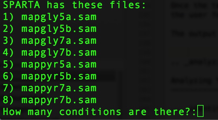
At the prompt that says:
How many conditions are there?:
Type:
4
Hit Enter/Return. There are 4 experimental conditions that we are considering:
- Glycerol pH 7.0
- Glycerol pH 5.7
- Pyruvate pH 7.0
- Pyruvate pH 5.7
Each condition has 2 replicates. The next prompt will read:
Enter the relevant file names, based on the names given in 'SPARTA has these files', with the replicates separated by a comma.
As an example, please see the 'conditions_input_example.txt' in the DEanalysis folder.
Once you have entered the file names, hit Enter/Return:
At this point, we need to edit a text file (conditions_input.txt) to tell SPARTA which file belongs to a given condition. To do this:
- Navigate to the SPARTA output folder called RNAseq_Data located on the desktop
- Go to the current run folder (will be the last folder listed if sorted by name)
- Go into the DEanalysis folder
- Open the conditions_input.txt file in a text editor (NOT MICROSOFT WORD) such as gedit
The number of experimental conditions listed are based on the number entered at the prompt asking “How many conditions are there?:”. Thus, in our case, there are 4. The contents of the file will look like:
Reference_Condition_Files:
Experimental_Condition_2_Files:
Experimental_Condition_3_Files:
Experimental_Condition_4_Files:
We now need to enter the file names of the replicates in each condition. These are comma-separated file names that correspond to the output given by SPARTA (denoted with red bracket)
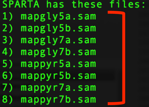
Note
The file names are case-sensitive and must be spelled exactly as listed in the output given by SPARTA
Thus, when all the file names are inputed, the conditions_input.txt file should look like this:
Reference_Condition_Files: mapgly7a.sam, mapgly7b.sam
Experimental_Condition_2_Files:mapgly5a.sam, mapgly5b.sam
Experimental_Condition_3_Files:mappyr7a.sam, mappyr7b.sam
Experimental_Condition_4_Files:mappyr5a.sam, mappyr5b.sam
Now, save the changes by going to File -> Save. Go back to the terminal and hit Enter/Return. From here, the workflow will perform the differential gene expression analysis through edgeR. If a batch effect may be present, the output will attempt to warn the user of the potential, unintended variable that must be accounted for before drawing experimental conclusions.
All the differential gene expression output is located in the RNAseq_Data -> date of your current run -> DEanalysis folder. The file output includes:
- Differential gene expression tables
- MDS plot (somewhat analogous to a principle component analysis plot) which will show whether your replicates group together and treatment groups separate based on the treatment
- BCV plot (biological coefficient of variation) to look at gene level variation between samples
Congratulations! You’ve analyzed RNA-seq data from raw reads to differential gene expression!
Analyzing Your Data
If you haven’t already, we recommend working through the example data analysis first before attempting to work through your own data set to familiarize yourself with the workflow.
As stated in the Introduction, SPARTA expects either compressed (.gz) or uncompressed FASTQ files (.fq or .fastq) as input, with a reference genome file in FASTA format and a genome feature file (.gtf) within the folder that contains the input data on your desktop. To see an example of appropriate input data, look inside the ExampleData folder within the SPARTA_Mac-master folder.
Now, to analyze your own data, follow the steps to initialize SPARTA, and start the analysis!
If you would like to tweak the analysis options for a given step/tool, have a look at the Altering Workflow Execution Options.
Identifying Potential Batch Effects
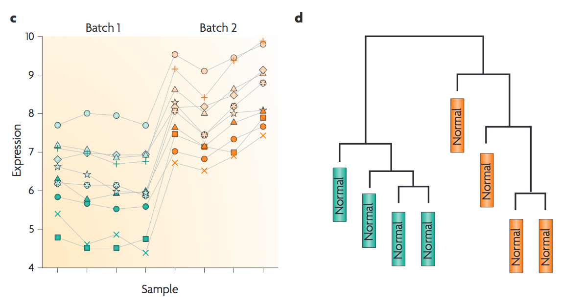
Batch effects can be a source of variation in RNA-seq data that can confound biological conclusions. In fact, there have been documented cases of batch effects present in published studies that led readers to be concerned for the validity of the results.
To quote a previously published paper in Nature Reviews Genetics, “Batch effects are sub-groups of measurements that have qualitatively different behaviour across conditions and are unrelated to the biological or scientific variables in a study. For example, batch effects may occur if a subset of experiments was run on Monday and another set on Tuesday, if two technicians were responsible for different subsets of the experiments or if two different lots of reagents, chips or instruments were used.”
Thus, it is paramount that one address batch effects within their data before drawing biological conclusions from a specific RNA-seq experiment. To illustrate what a batch effect may look like within the data, we will utilize several different plots.
This first plot comes from the Nature Reviews Genetics paper where they examine Affymetrix data from a published bladder cancer study. You can quickly see that panels C and D from Figure 1 show that samples from batch 1 (blue) cluster together based on gene expression and samples from batch 2 (orange) cluster together.
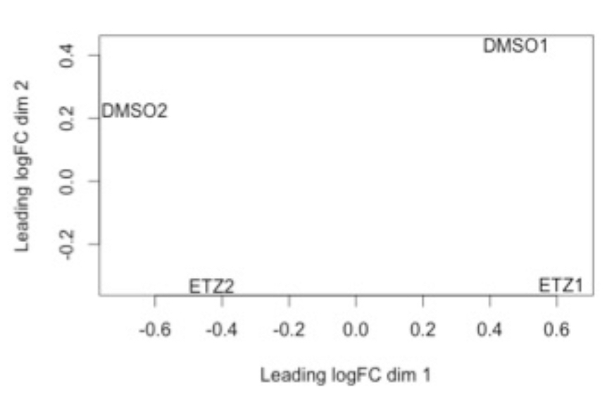
Within RNA-seq data, using SPARTA and the MDS plot generated by edgeR, another example of batch effects within a study comparing Mycobacterium tuberculosis treated with a compound, we can clearly see that the mock-treated samples (DMSO) and compound-treated samples (ETZ) separate based on batch (A vs B) instead of by treatment. Ideally, we would have the samples group together based on treatment as opposed to batch.
If a potential batch effect is detected in the data set, SPARTA will output a message into the terminal that says:
IMPORTANT! YOU MAY HAVE A BATCH EFFECT! PLEASE LOOK AT THE MDS PLOT!
If this occurs, have a look at the MDS plot in the RNAseq_Data folder -> date of current run -> DEanalysis folder -> MDSplot.png
From here, you will want to adjust your model to account for the batch effect. Within edgeR, this can be accomplished through an additive linear model. The documentation for edgeR contains a tutorial on how to deal with batch effects that can be found here.
Future implementations of SPARTA will include the ability to adjust for batch effects.
Altering Workflow Execution Options
SPARTA is capable of allowing the user to alter the parameters associated with each analysis step to be tailored to specific use cases. Below are the different parameters that can be altered and their usage.
Options:
Usage: python SPARTA.py [options]

      Simple Program for Automated reference-based bacterial RNA-seq Transcriptome
      Analysis (SPARTA)

-h, --help            show this help message and exit
--cleanup             Clean up the intermediate files to save space. Default
                      action is to retain the intermediate files.
--verbose             Display more output for each step of the analysis.
--noninteractive      Non-interactive mode. This is for running SPARTA
                      without any user input. Assumes data is on the
                      desktop. If this option is specified, you must fill
                      out the configuration file (ConfigFile.txt) with the
                      appropriate experimental conditions in the SPARTA
                      folder.
--threads=THREADS     Define the number of threads that SPARTA should run
                      with. This will enable some speed-up on multi-
                      processor machines. As a generality, define the number
                      of threads as the same number of cores in your
                      computer. Default is 2.

Trimmomatic options:
  The order the options will be run are: ILLUMINACLIP, LEADING,
  TRAILING, SLIDINGWINDOW, MINLEN

  --clip=ILLUMINACLIP
                      ILLUMINACLIP options. MiSeq & HiSeq usually
                      TruSeq3.fa; GAII usually TruSeq2.fa. Default is
                      ILLUMINACLIP:TruSeq3-SE.fa:2:30:10. Usage:
                      --clip=<adapterseqs>:<seed mismatches>:<palindrome
                      clip threshold>:<simple clip threshold>
  --lead=LEADING      Set the minimun quality required to keep a base.
                      Default is LEADING=3. Usage: --lead=<quality>
  --trail=TRAILING    Set the minimum quality required to keep a base.
                      Default is TRAILING=3. Usage: --trail=<quality>
  --slidewin=SLIDINGWINDOW
                      SLIDINGWINDOW options. Default is SLIDINGWINDOW:4:15.
                      Usage: --slidewin=<window_size>:<required_quality>
  --minlentrim=MINLENTRIM
                      Set the minimum read length to keep in base pairs.
                      Default is 36. Usage: --minlentrim=<readlength>

Bowtie options:
  --mismatch=MISMATCH
                      Output alignments with at most a defined number of
                      mismatches. Usage: --mismatch=<integer_value>
  --otherbowtieoptions=OTHERBOWTIEOPTIONS
                      Bowtie has so many options that it is not worth
                      listing them here. Go to http://bowtie-
                      bio.sourceforge.net/manual.shtml#command-line for the
                      manual and all available options. Usage:
                      --otherbowtieoptions='all options inputed as a string
                      (note the quotes!)'

HTSeq options:
  --stranded=STRANDED
                      Stranded options: yes, no, reverse. Default is
                      --stranded=reverse. Usage: --stranded=yes/no/reverse
  --order=ORDER       Order options: name, pos. Usage: --order=name/pos.
  --minqual=MINQUAL   Skip all reads with quality lower than the given
                      value. Default is --minqual=10. Usage:
                      --minqual=<value>
  --type=TYPE         The feature type (3rd column in GTF file) to be used.
                      Default is --type=exon (suitable for RNA-seq analysis)
  --idattr=IDATTR     Feature ID from the GTF file to identify counts in the
                      output table Default is --idattr=gene_id. Usage:
                      --idattr=<id attribute>
  --mode=MODE         Mode to handle reads overlapping more than one
                      feature. Default is --mode=union. Usage: --mode=union
                      /intersection-strict/intersection-nonempty